Tuesday, August 6, 2019

Bary: The Barycentric Interpolation in MatLab


Purpose
  • The library "Bary" provides MatLab functions for the barycentric interpolation.

Click Here to Download the Codes


Specifications
  • Name:Bary
  • Author: Feng Chen
  • Version: 1.0
  • Language: MATLAB

Simple Example
  • Equation: \begin{equation} \begin{aligned} &c_1(x)u''(x)+ c_2(x)u'(x)+c_3(x)u(x) = f(x), \quad \Omega = (a,b),\\ &u \text{ satisifies the general boundary condition}. \end{aligned} \end{equation}
  • Parameters: \begin{equation} c_1(x)=-4x^2, \quad c_2(x) = 3x, \quad c_3(x)=2. \end{equation}
  • Exact solution and input functions: \begin{equation} u(x) = \sin x , \end{equation} then $f(x)$ is calculated accordingly.

Quick Start
  • Compiling and running:
    matlab test_bvp
    
  • Output:
     
    error =
    
       1.1180e-13
    
  • CPU: Intel(R) Core(TM) i5-4590S CPU @ 3.00GHz
  • OS: Ubuntu 18.04.
  • Release: MATLAB R2019a.

References
  • Tee, T. & Trefethen, L. A Rational Spectral Collocation Method with Adaptively Transformed Chebyshev Grid Points, SIAM Journal on Scientific Computing, Volume 28, Number 5, 1798-1811, (2006).

Core Subroutines
    
    
    function [P L U A] = bc_bvp_matrix(c1, c2, c3, a1, a2, b1, b2, D1, D2)
    
    n = length(c1);
    A = diag(c1)*D2 + diag(c2)*D1 + diag(c3);
    A(1,:) = a1*[1 zeros(1,n-1)] + b1*D1(1,:);
    A(n,:) = a2*[zeros(1,n-1) 1] + b2*D1(n,:);
    [L,U,P] = lu(A); 


Wednesday, January 23, 2019

FFTM: Fourier Spectral Methods in MATLAB


Purpose
  • The library "fftm" provides MatLab functions that are useful for solving ellipitic systems in 1D and 2D with Fourier spectral methods. It works for both complex and real data.

Click Here to Download the Codes


Specifications
  • Name:fftm
  • Author: Chris Chen
  • Version: 2.2
  • Language: MATLAB

Simple Example
  • Equation: \begin{equation} \begin{aligned} &a(x) u - b(x) (\beta_1 u_{xx} + \beta_2 u_{yy}) = f, \quad \Omega = (0,2\pi)^2,\\ &u \text{ is periodic}. \end{aligned} \end{equation}
  • Parameters: \begin{equation} a(x) =-0.1+\sin x + \cos 2y, \quad b(x) = 4 + \cos x + \sin y, \quad \beta_1=2, \quad \beta_2=3. \end{equation}
  • Exact solution and input functions: \begin{equation} u(x,y) = (1+\sin x + 2\cos y)(2+ \cos y), \end{equation} then $f(x,y)$ is calculated accordingly.

Quick Start
  • Compiling and running:
    matlab test_rfft_elliptic_solver_2dv
    
  • Output:
     
    bicgstab converged at iteration 10.5 to a solution with relative residual 8.5e-11.
    
    err =
    
         5.548761450313577e-10
    
  • CPU: Intel(R) Xeon(R) CPU X5550 @2.67GHz.
  • OS: CentOS release 6.4 (Final).
  • Release: MATLAB R2012a.

References
  • Fast Fourier transform in MATLAB. Link.

Core Subroutines
    
    %fftr_modes returns the ordering
    %of the wave number when the input data in 
    %the physical space are real numbers.
    %High dimensional index is the tensor 
    %product of 1-D indices.
    %The orderings are different for odd k 
    %and even k.
    
    %k contains the ordering.
    %m is the highest mode.
    function [lk m] = fftr_modes(n)
    
    
    lk = zeros(n,1); 
    
    m = floor((n-1)/2);
    
    lk(1:m+1) = [0:m]'; 
    
    lk(n:-1:n-m+1) = -[1:m]';


Sunday, September 23, 2018

Alpha-BS: A MATLAB Package of Mathematical Algorithms for the Black-Scholes Model


Purpose
  • The library "alpha-bs" computes the approximation to classic and fractional Black-Scholes models for European and American options, with finite difference method, spectral method, backward Euler method, BDF2 method, Crank-Nicolson method, projected LU method, and operator splitting method.

Click Here to Download the Codes


Simple Example
  • Equation: \begin{equation} \begin{aligned} & v_t = \frac{\sigma^2 s^2}{2} v_{ss} + (r-q) s v_s - rv, \quad (s,t) \in (0,\infty) \times (0,T],\\ & v(s,0) = g(s). \end{aligned} \end{equation}
  • Parameters: \begin{equation} T =0.25, \quad r= 0.05, \quad \sigma=0.15, \quad K=50, \quad q =0, \quad S_m = 2K. \end{equation}
  • Exact solution for European options: \begin{equation} \begin{aligned} & C = Se^{-q(T-t)} N(d_1) - Ke^{-r(T-t)} N(d_2), \\ & P = Ke^{-r(T-t)} N(-d_2)-Se^{-q(T-t)}N(-d_1), \end{aligned} \end{equation} where \begin{equation} \label{x1} d_1 = \frac{\ln(S/K) +(T-t)(r-q+\frac{\sigma^2}{2})}{\sigma \sqrt{(T-t)}}, \quad d_2 = d_1 -\sigma \sqrt{(T-t)}. \end{equation} In the above, $S$ is the stock price, $K$ is the strike price, $r$ is the interest rate, $q$ is the dividend rate, $T$ is the maturity span of the option, and $t$ is the spot time (e.g., $t=0$ indicates the present time). And $N(x)$ is the cumulative distribution function (cdf) of a standard normal random variable: \begin{equation} \label{Nx} N(x) = \frac{1}{\sqrt{2\pi}} \int_{-\infty}^x e^{-\frac{s^2}{2}} ds. \end{equation}

Quick Start
  • Compiling and running:
    matlab test_bs_eu
    
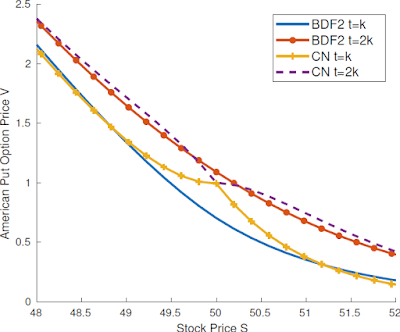
  • Example Output for American options:


  • CPU: Intel(R) i5-4310U.
  • OS: Windows Home 10.
  • Release: MATLAB R2017b.

References
  • A new operator splitting method for American options under fractional black–scholes models Chris Chen, Zeqi Wang, Yue Yang, Computers & Mathematics with Applications 77 (8), 2130-2144, 2019
  • A new spectral element method for pricing European options under the Black–Scholes and Merton jump diffusion models, Feng Chen, Jie Shen, Haijun Yu, Journal of Scientific Computing 52 (3), 499-518, 2012
  • Operator splitting methods for American option pricing, Samuli Ikonen, Jari Toivanen, Applied mathematics letters 17 (7), 809-814

Code Highlights
    
    % Backward Euler's method for the Black-Scholes Eqaution
    [v vq] = mch_bs_eu_be(pid, N, M, M, K, T, r, sigma, q, S, g, Sq);
    % BDF2 method for the Black-Scholes Eqaution
    [v vq] = mch_bs_eu_bdf2(pid, N, M, K, T, r, sigma, q, S, g, Sq);
    % Crank-Nicolson method for the Black-Scholes Eqaution
    [v vq] = mch_bs_eu_cn(pid, N, M, 4, K, T, r, sigma, q, S, g, Sq);


Wednesday, July 24, 2013

VERLET: Symplectic integration for Hamiltonian systems and adjoint solvers


Purpose
  • The package "Verlet" solves the second-order differential equation (or a Hamiltonian system) with the velocity Verlet scheme. It is second-order accurate in both position and velocity. In addition, the velocity Verlet scheme almost preserves the Hamiltonian (oscillating around a constant mean). The package also provides the corresponding adjoint solver.

Specifications
  • Name: Verlet.
  • Author: Feng Chen.
  • Finishing date: 07/24/2013.
  • Languages: MATLAB.

Simple Example
  • Equation: \begin{equation} \begin{aligned} & u''=\lambda u, \quad t \in (0,T],\\ & u(0) = 0, \quad u'(0) = \sqrt{-\lambda}. \end{aligned} \end{equation}
  • Parameters: \begin{equation} T=10, \quad \lambda=-400, \quad \delta t = 0.0001. \end{equation}
  • Exact solution: \begin{equation} u(t) = \sin(\sqrt{-\lambda} t). \end{equation}

Quick Start
  • Compiling and running:
    matlab Verlet_Driver
    
  • Output:
    maximum error of position and velocity =
         5.821930990741464e-04
    
  • CPU: Intel(R) Xeon(R) CPU X5550 @2.67GHz.
  • OS: CentOS release 6.4 (Final).
  • Release: MATLAB R2012a.

References
  • Verlet integration. Link.

Code Highlights
    
    % the velocity-Verlet time stepping.
    
    K = -lambda;
    
    r = u0(1);
    v = u0(2);
    a = -K*r;
    
    for i = 1:nt
     rt = r; 
     r = (1-K*dt*dt/2)*r + dt*v; 
     v = (1-K*dt*dt/2)*v + dt*(K*dt*dt/4-1)*K*rt; 
    end
    u = [r; v];


Thursday, July 11, 2013

AGATE: GPU-accelerated 3-D Chebyshev collocation methods for elliptic equations


Purpose
  • The package "Agate" provides a GPU-accelerated Chebyshev collocation method for solving the single elliptic equation with Dirichlet, Neumann, or Robin boundary conditions on a 3-D rectangular domain.

Specifications
  • Name: Agate.
  • Author: Feng Chen.
  • Finishing date: 05/30/2013.
  • Languages: CUDA C++, Fortran 90.
  • Required libraries: BLAS, LAPACK, CUBLAS.

Simple Example
  • Equation: \begin{equation} \begin{aligned} & \alpha u -(\beta_1 u_{xx} + \beta_2 u_{yy} + \beta_3 u_{zz}) = f, &&\quad \text{in } \Omega, \\ & au + b\frac{\partial u}{\partial \boldsymbol{n}} = c, && \quad \text{on } \partial \Omega. \end{aligned} \end{equation}
  • Parameters: \begin{equation} \Omega = (-1,1)^3 , \quad \alpha =2, \quad \beta_1=3, \quad \beta_2=4, \quad \beta_3 = 5, \quad a = 1, \quad b=1. \end{equation}
  • Exact solution and input functions: \begin{equation} u(x,y,z) = e^{x+y+z}, \end{equation} then $f(x,y,z)$ and $c(x,y,z)$ are calculated accordingly.

Quick Start
  • Compiling and running:
    cd ./Agate
    make library
    nvcc Agate_Main.cu -llibrary -llapack -lblas
    ./a.out
    
  • Output:
    Nx = 2^5, Ny = 2^6, Nz = 2^7
    Device 0: Tesla M2050 of version 2.0
    intialization time: 0.0961988
    cpu time bulk: 0.110826
    cpu error bulk: 1.57341e−11
    cpu error upx: 1.53673e−11
    cpu error umx: 3.08875e−12
    cpu error upy: 1.48668e−11
    cpu error umy: 2.78527e−12
    cpu error upz: 1.2097e−11
    cpu error umz: 1.57017e−11
    cpu error du: 2.71758e−10
    gpu time HtD: 0.00597085
    gpu time bulk: 0.00152022
    gpu time BV: 0.000412896
    gpu time diff: 0.00107117
    gpu time DtH: 0.00265923
    gpu error bulk: 1.57332e−11
    gpu error upx: 1.53664e−11
    gpu error umx: 3.08864e−12
    gpu error upy: 1.48654e−11
    gpu error umy: 2.78522e−12
    gpu error upz: 1.2097e−11
    gpu error umz: 1.57021e−11
    gpu error du: 2.71349e−10
    ...
    
  • CPU: Intel(R) Xeon(R) CPU X5630 @2.53GHz.
  • GPU: Nvidia Tesla M2050.
  • OS: CentOS release 6.4 (Final).
  • Compiler: nvcc 4.2.9, gcc/gfortran 4.5.1.

References
Code Highlight
    
    // 
    // Mars_D_Invert performs the inversion in the frequency space
    // on the device.
    //
    // Input:
    //        dd: structure for static data
    //        alpha, beta: coefficient
    //        d_f: right hand side
    // Output:
    //        d_f: solution
    // Other:
    //        lambda: eigenvalue
    //        s: stiffness matrix
    //        q: number of quadrature points
    //
    inline void Mars_D_Invert (Mars& dd, double alpha, 
     double betax, double betay, double betaz, double* d_f, double* wk) {
     dim3 T(8, 8, 8);  
     dim3 B((dd.qx+7)/8, (dd.qy+7)/8, (dd.qz+7)/8);
     Mars_Kernel <<<B,T>>> (alpha, betax, betay, betaz, 
      dd.qx, dd.qy, dd.qz, dd.lambdax, dd.lambday, dd.lambdaz, wk, d_f);    
    }


Sunday, July 7, 2013

BARIS: Fourier method for the Burgers' equation


Purpose
  • The package "BariS" solves the 1-D viscous Burgers' equation with periodic boundary condition. The spatial discretization is a Fourier psuedospectral method. Three methods were proposed to calculate the nonlinear term: (i) evaluating Fourier coefficients exactly with the convolution; (ii) padding zeros in the $k$-space; and (iii) filtering with the two thirds rule. For the temporal discretization, a second-order symmetric Strang splitting was used. The linear diffusion term was integrated exactly, while the nonlinear term by a third-order Runge-Kutta scheme.

Specifications
  • Name: BariS.
  • Author: Feng Chen.
  • Finishing date: 10/13/2012.
  • Languages: MATLAB.

Simple Example
  • Equation: \begin{equation} \begin{aligned} & u_t + uu_x = \epsilon u_{xx}, \quad x\in (0,2\pi), \\ & u \text{ is periodic}. \end{aligned} \end{equation}
  • Parameters: \begin{equation} T=2, \quad \epsilon=0.001, \quad N_x = 1024, \quad \delta t = 0.005. \end{equation}
  • Initial condition: \begin{equation} u_0(x) = \sin(x). \end{equation}

Quick Start
  • Compiling and running:
    matlab Bari_Driver_Serial
    
  • Graphics:
  • CPU: Intel(R) Xeon(R) CPU X5550 @2.67GHz.
  • OS: CentOS release 6.4 (Final).
  • Release: MATLAB R2012a.

References
Code Highlights
    
    %%% calculate the nonlinear term with convolution 
    
    % re-order the modes
    uu = [ui(lcut+1:N); ui(1:lcut)]/N;
    
    % convolution
    uc = conv(uu,uu);
    
    % re-order to matlab convention
    m = length(uc);
    ucc = [uc((m+1)/2:m); uc(1:(m-1)/2)]*2*N;
    
    % first-order derivative
    du = rfft_grad_1d(ucc, 1);
    
    % cut off the high modes
    rhs = [du(1:lcut); du(lcut+N:m)]/2;
    rhs = -rhs/2;


Saturday, July 6, 2013

FITZ: Parallel integration for FitzHugh-Nagumo ODEs


Purpose
  • The package "Fitz" solves the FitzHugh-Nagumo equation using the parareal method. To construct serial solvers with coarse and fine resolutions, the first-order forward Euler scheme was used.

Specifications
  • Name: Fitz.
  • Author: Feng Chen.
  • Finishing date: 07/06/2013.
  • Languages: MATLAB.

Simple Example
  • Equation: \begin{equation} \begin{aligned} & v' = v-v^3-w+I_{\text{ext}},\\ & \tau w' = v + a - bw. \end{aligned} \end{equation}
  • Parameters: \begin{equation} I_{\text{ext}}=0.5, \, a=0.7,\, b=0.8, \,\tau=12.5,\, T=200, \,\Delta T =0.1, \, \Delta t = 0.05, \, \delta t=0.001. \end{equation}
  • Initial conditions: \begin{equation} v(0)=1, \quad w(0)=0. \end{equation}

Quick Start
  • Compiling and running:
    matlab Fitz_Driver_Parareal
    
  • Output:
    iteration 0, 0.000000e+00, 7.040824e-01 
    iteration 1, 1.235809e-02, 6.917243e-01 
    iteration 2, 8.904816e-04, 6.908338e-01 
    iteration 3, 6.172277e-05, 6.907721e-01 
    iteration 4, 2.008283e-06, 6.907701e-01 
    iteration 5, 9.682426e-08, 6.907702e-01 
    iteration 6, 2.131734e-08, 6.907702e-01 
    iteration 7, 2.023203e-09, 6.907702e-01 
    iteration 8, 1.402405e-10, 6.907702e-01 
    iteration 9, 7.806200e-12, 6.907702e-01 
    iteration 10, 3.443912e-13, 6.907702e-01 
    sucessful return! 
    ...
    
  • Graphics:
  • CPU: Intel(R) Xeon(R) CPU X5550 @2.67GHz.
  • OS: CentOS release 6.4 (Final).
  • Release: MATLAB R2012a.

References
Code Highlights
    
    % parareal iteration
    for k = 2:imax+1
     % fine solver
     for i = k:n+1
      ytF = Fitz_Time(sF, yp(:,i-1), l*m); yF(:,i) = ytF(:,end);
     end
     
     % coarse solver
     yc(:,k) = yF(:,k); 
     for i = k+1:n+1
      ytG = Fitz_Time(sG, yc(:,i-1), m); yGc(:,i) = ytG(:,end);
      yc(:,i) = yF(:,i) + yGc(:,i) - yGp(:,i); 
     end
      
      % check errors
     ed = abs(yc(1,end)-yp(1,end));  % relative error
     et = abs(ye(1,end)-yc(1,end));  % true error
     fprintf('iteration %d, %e, %e \n', k-1, ed, et);  
    
     % check convergence
     if (ed < tol)
      fprintf('sucessful return! \n');
      break
     end
    
     % update solution
     yGp(:,k:n+1) = yGc(:,k:n+1); 
     yp(:,k:n+1) = yc(:,k:n+1); 
    end